Shrinkage

Here we apply the Shrinkage methods (Ridge regression and lasso) to the Hitters data. The dataset is available in the R package, ISLR.

1 Data info

We wish to predict a baseball player’s Salary on the basis of various statistics associated with performance in the previous year.

library(ISLR)
names(Hitters)

 [1] "AtBat"     "Hits"      "HmRun"     "Runs"      "RBI"       "Walks"    
 [7] "Years"     "CAtBat"    "CHits"     "CHmRun"    "CRuns"     "CRBI"     
[13] "CWalks"    "League"    "Division"  "PutOuts"   "Assists"   "Errors"   
[19] "Salary"    "NewLeague"

dim(Hitters)

[1] 322  20

Some salary data are missing in the dataset, which are represented as NA in R. In that case, most operations on Salary will also return NA:

mean(Hitters$Salary)

[1] NA

The na.omit() function removes all of the rows that have missing values in any variable:

Hitters=na.omit(Hitters)
dim(Hitters)

[1] 263  20

mean(Hitters$Salary)

[1] 535.9259

2 glmnet

We will use the glmnet package in order to perform ridge regression and the lasso. The main function in this package is glmnet(), which can be used to fit ridge regression models, lasso models, and more.

This function has slightly different syntax from other model-fitting functions that we have encountered. In particular, we must pass in an x matrix as well as a y vector, and we do not use the y ∼ x syntax.

We will now perform ridge regression and the lasso in order to predict Salary on the Hitters data.

x = model.matrix(Salary ~ ., Hitters)[,-1]
y = Hitters$Salary

The model.matrix() function is particularly useful for creating x; not only does it produce a matrix corresponding to the 19 predictors, but it also automatically transforms any qualitative variables into dummy variables.

The latter property is important because glmnet() can only take numerical, quantitative inputs.

3 Ridge regression

The glmnet() function has an alpha argument that determines what type of model is fit.

• If alpha=0, then a ridge regression model is fit;
• if alpha=1, then a lasso model is fit.

We first fit a ridge regression model.

library(glmnet)
grid = 10^seq(10,-2,length=100)
ridge.mod = glmnet(x,y,alpha=0,lambda = grid)

By default, the glmnet() function performs ridge regression for an automatically selected range of $λ$ values. However, here we have chosen to implement the function over a grid of values ranging from $λ = 10^{10}$ to $λ = 10^{−2}$.

By default, the glmnet() function standardizes the variables so that they are on the same scale. This can be expected as we always scale the data first before performing lasso or ridge regrression.

Associated with each value of $λ$ is a vector of ridge regression coefficients, stored in a matrix that can be accessed by coef().

dim(coef(ridge.mod))

[1]  20 100

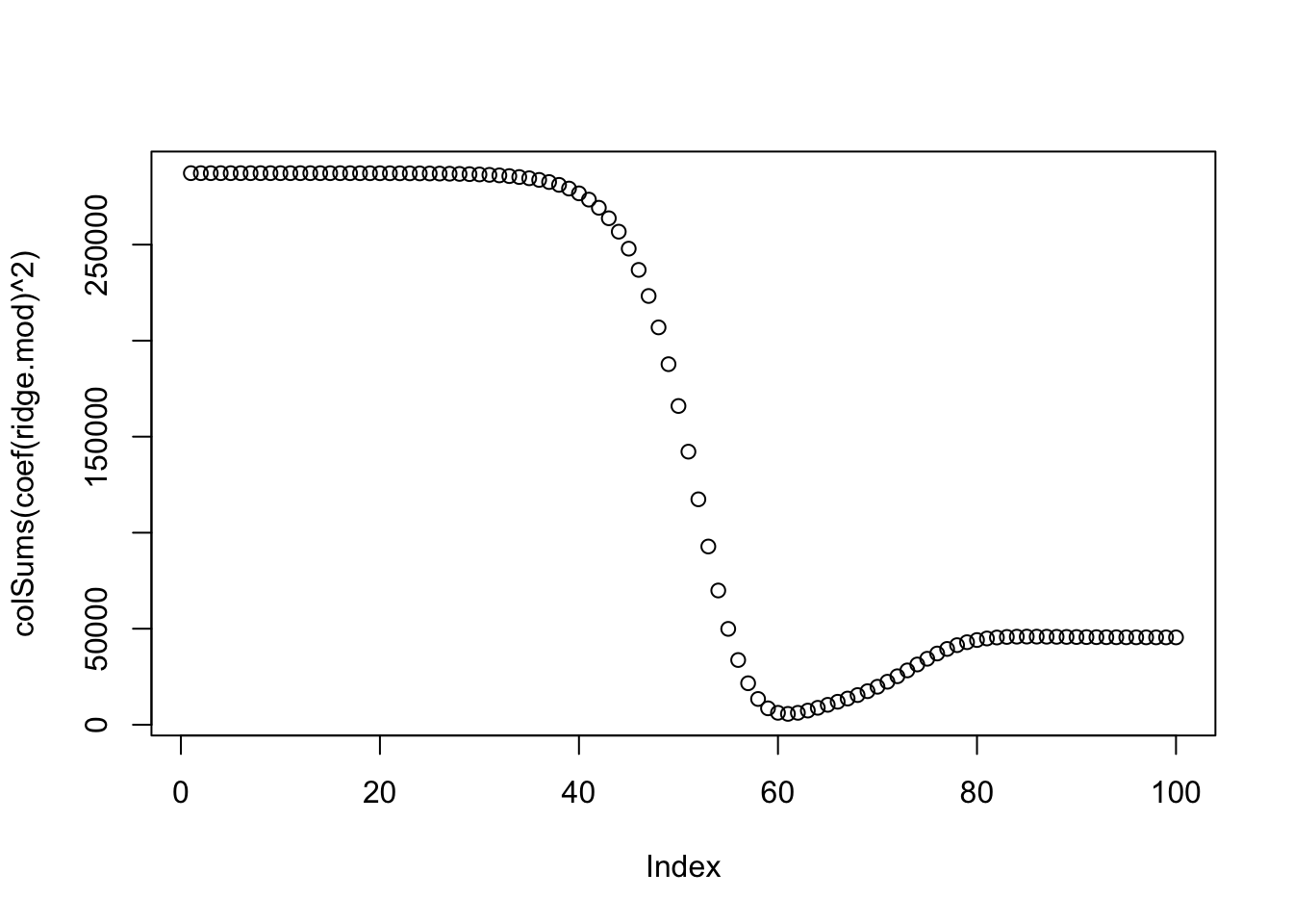
When a large $λ$ is used, we expect the coefficient estimates to be much smaller, in terms of $\ell_2$ norm.

plot(colSums(coef(ridge.mod)^2))

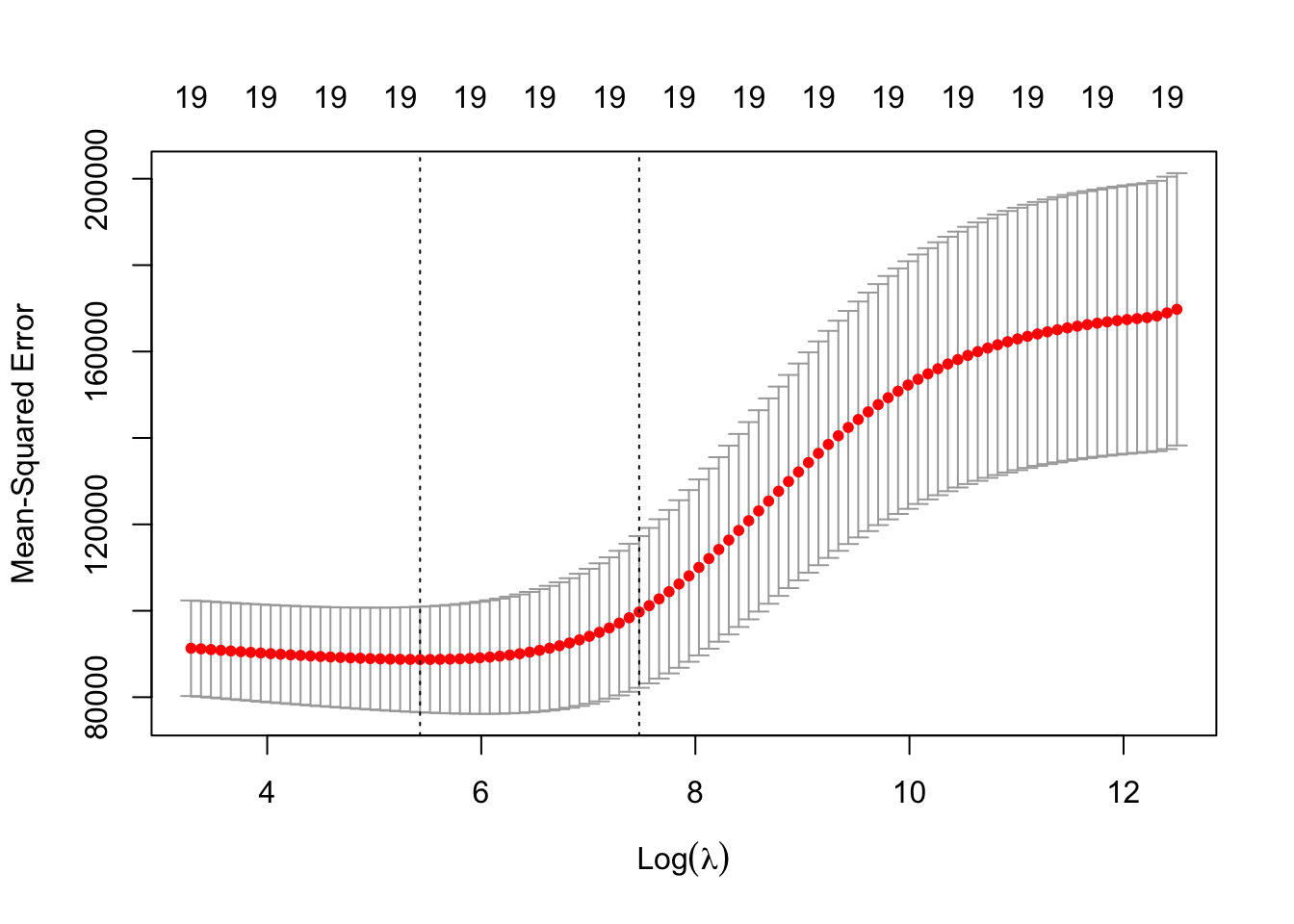
4 Cross-validation

We need to do cross-validation to select the tuning parameter $\lambda$. To do that, We can use the built-in cross-validation function, cv.glmnet().

By default, the function performs ten-fold cross-validation. This can be changed using the argument nfolds.

Note that we set a random seed first so our results will be reproducible, since the choice of the cross-validation folds is random.

train = sample(1:nrow(x), nrow(x)/2)
test = (-train)
y.test = y[test]

set.seed (1)
cv.out = cv.glmnet(
  x[train,],
  y[train],
  alpha=0)
plot(cv.out)

bestlam = cv.out$lambda.min
bestlam

[1] 227.7175

What is the test MSE associated with this value of lambda?

ridge.pred = predict(
    ridge.mod,
    s = bestlam,
    newx = x[test,])
mean((ridge.pred-y.test)^2)

[1] 131513.3

As comparison, the test MSE using LS is:

lm1 = lm(y ~ x, subset = train)
lm.pred = predict(
    lm1,
    newx=x[test,])
mean((lm.pred - y[test])^2)

[1] 320399.7

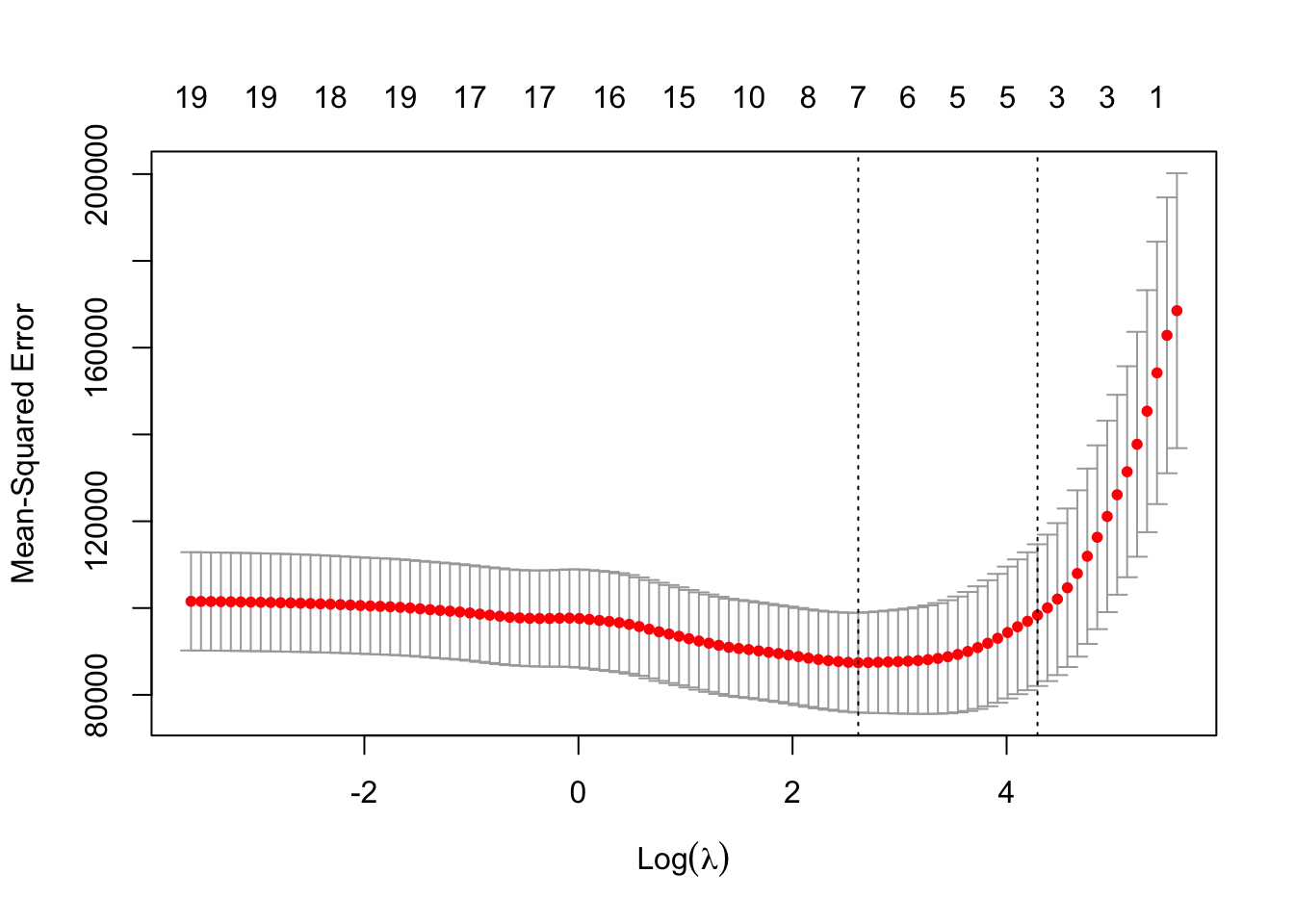
Finally, we refit our ridge regression model on the full data set, using the value of $λ$ chosen by cross-validation, and examine the coefficient estimates.

predict(
  glmnet(x,y,alpha=0),
  type="coefficients",
  s=bestlam)[1:20,]

 (Intercept)        AtBat         Hits        HmRun         Runs          RBI 
 10.12543477   0.04073623   0.98100058   0.22091888   1.10583995   0.87494642 
       Walks        Years       CAtBat        CHits       CHmRun        CRuns 
  1.77270895   0.36287096   0.01120584   0.06354969   0.44371404   0.12634936 
        CRBI       CWalks      LeagueN    DivisionW      PutOuts      Assists 
  0.13441311   0.03386753  26.30573173 -89.63307532   0.18742083   0.04001428 
      Errors   NewLeagueN 
 -1.73395456   7.65380522 

As expected, none of the coefficients are zero, since ridge regression does not perform feature selection.

5 Lasso

The process of performing a lasso fit is almost the same, except that we use the argument alpha=1.

lasso.mod = glmnet(
    x[train ,],
    y[train],
    alpha=1,
    lambda=grid)

plot(lasso.mod)

Warning in regularize.values(x, y, ties, missing(ties), na.rm = na.rm):
collapsing to unique 'x' values

We now perform cross-validation and compute the associated test error.

set.seed(1)
cv.out = cv.glmnet(
    x[train ,],
    y[train],
    alpha=1)
plot(cv.out)

bestlam = cv.out$lambda.min
lasso.pred = predict(
    lasso.mod,
    s=bestlam,
    newx=x[test,])
mean((lasso.pred-y.test)^2)

[1] 149374.9

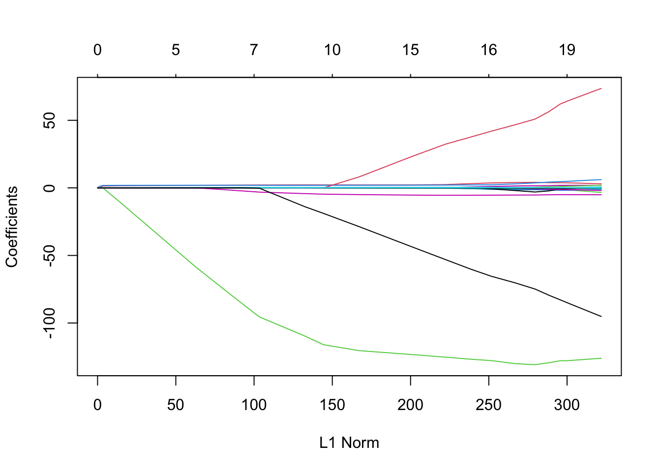
This is similar to the test MSE of ridge regression with λ chosen by cross-validation. However, the lasso has a substantial advantage over ridge regression in that the resulting coefficient estimates are sparse.

Here we see that 12 of the 19 coefficient estimates are exactly zero. So the lasso model with λ chosen by cross-validation contains only seven variables.

lasso.coef = predict(
    glmnet(x,y,alpha=1,lambda=grid),
    type="coefficients",
    s=bestlam)[1:20,]
lasso.coef

  (Intercept)         AtBat          Hits         HmRun          Runs 
 8.970813e+00  0.000000e+00  1.917459e+00  0.000000e+00  0.000000e+00 
          RBI         Walks         Years        CAtBat         CHits 
 0.000000e+00  2.249694e+00  0.000000e+00  0.000000e+00  0.000000e+00 
       CHmRun         CRuns          CRBI        CWalks       LeagueN 
 9.196017e-04  2.089282e-01  4.181784e-01  0.000000e+00  8.973648e+00 
    DivisionW       PutOuts       Assists        Errors    NewLeagueN 
-1.090652e+02  2.276060e-01  0.000000e+00 -9.684873e-02  0.000000e+00