Trees

Hunan U

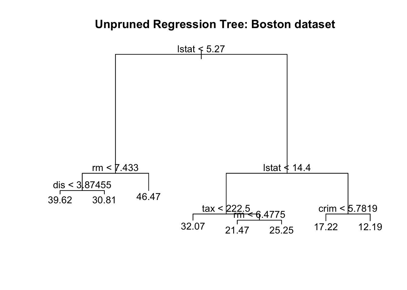
我们仍以 Boston 数据集为例来演示树方法, 先加载包 MASS.

library(MASS)

你可以运行 ?MASS::Boston 来回顾关于 Boston 数据集的说明.

`tree` 包

tree 包提供的 tree 函数, 可用于构建回归树.

library(tree)

我们随机抽取一半的数据作为训练集, 并用训练集中的数据来”种树” (fit the tree).

set.seed(18)
boston_idx <- sample(1:nrow(Boston), nrow(Boston) / 2)
boston_trn = Boston[boston_idx,]
boston_tst = Boston[-boston_idx,]

boston_tree <- tree(medv ~ ., data = boston_trn)

函数 tree 的使用方法和我们熟悉的 lm 函数基本一致, 我们这里只用到了两个参数:

medv ~ .: 指定回归公式, 这里的被预测变量是房价 medv, 点号 . 说明其它的所有变量均被用于预测 medv
data = boston_trn: 指定训练集

所有的回归信息都储存在变量 boston_tree 中,

summary(boston_tree)


Regression tree:
tree(formula = medv ~ ., data = boston_trn)
Variables actually used in tree construction:
[1] "lstat" "rm"    "dis"   "tax"   "crim" 
Number of terminal nodes:  8 
Residual mean deviance:  12.2 = 2988 / 245 
Distribution of residuals:
     Min.   1st Qu.    Median      Mean   3rd Qu.      Max. 
-10.25000  -2.35500  -0.06778   0.00000   1.87700  15.31000

summary 函数的输出, 说明我们只用到了5个变量来种树, 重要性由高到低依次为: 社区富裕程度 (lstat, 值越小表示社区越富裕), 房间数 (rm), 到市中心距离 (dis), 房产税 (tax), 犯罪率 (crim).

我们仍然用 plot 函数来画这棵树:

plot(boston_tree)
text(boston_tree, pretty = 0)
title(main = "Unpruned Regression Tree: Boston dataset")

这个未剪枝的树共有8片叶子: $|T| = 8$ .

我们使用交叉验证来剪枝 (i.e., 挑选子树). 我们直接使用 cv.tree 函数来进行交叉验证:

boston_tree_cv = cv.tree(boston_tree)
plot(boston_tree_cv$size, sqrt(boston_tree_cv$dev / nrow(boston_trn)), type = "b",
     xlab = "Tree Size", ylab = "CV-MSE")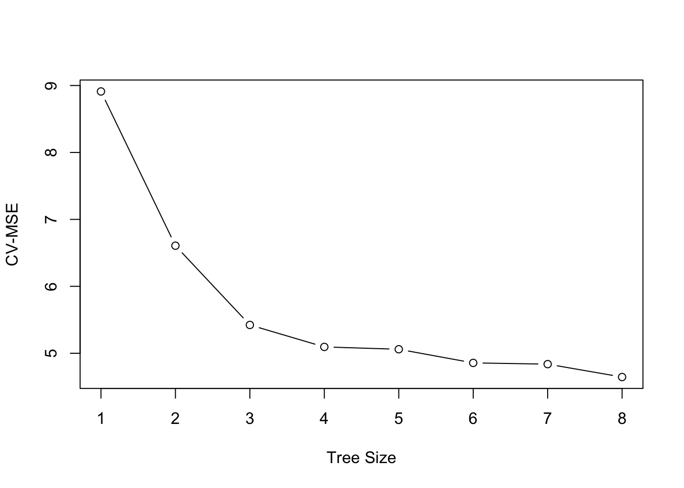

上图说明:

在Boston 数据集中, 最复杂的树 (i.e., tree size 为8)的预测效果是最好的.
如果你的主要目的是预测, 那么就没有必要进行剪枝. 不过, 实际中人们用单个回归树的目的往往不是预测, 而是因为单个回归树模型的结果很好解释.
出于”易于解释”的目的, 你可以挑选包含6片叶子的子树, 作为你的最终模型. 因为由图可知, 大小为6和大小为7的子树, 预测能力基本相同.

我们使用 prune.tree 函数来进行剪枝:

boston_tree_prune = prune.tree(boston_tree, best = 6)
summary(boston_tree_prune)


Regression tree:
snip.tree(tree = boston_tree, nodes = c(4L, 13L))
Variables actually used in tree construction:
[1] "lstat" "rm"    "tax"   "crim" 
Number of terminal nodes:  6 
Residual mean deviance:  14.64 = 3615 / 247 
Distribution of residuals:
   Min. 1st Qu.  Median    Mean 3rd Qu.    Max. 
-10.220  -2.438  -0.238   0.000   1.877  17.100

plot(boston_tree_prune)
text(boston_tree_prune, pretty = 0)
title(main = "Pruned Regression Tree")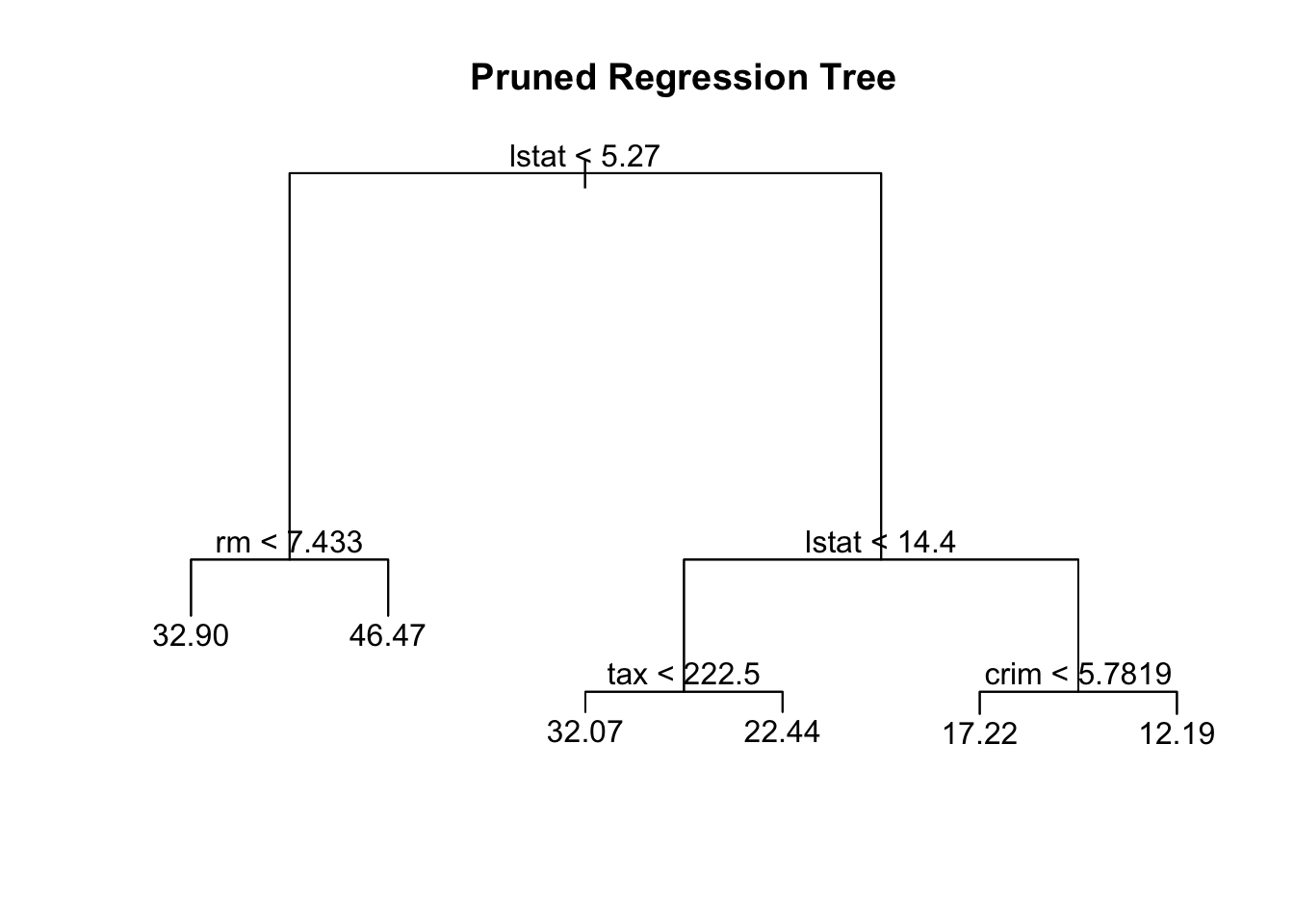

`rpart` 包

当我们使用tree 包来构建回归树时, 基本流程和之前的线性模型基本一致. 此外, tree 包提供的函数 cv.tree 和 prune.tree 使用十分方便, 适合用来快速构建回归树.

除了 tree 包外, 你还可以 rpart 包来构建回归树. rpart 包的功能更强大, 提供了更多关于成本复杂性和交叉验证的参数选项. 如果你需要对模型参数进行更精细的控制, 建议使用 rpart 包.

rpart 的全名是 “Recursive Partitioning And Regression Trees”.

library(rpart)

使用 rpart 函数来种树:

boston_tree = rpart(medv ~ ., data = boston_trn)
# summary(boston_tree)

我们使用rpart.plot包中的 prp 函数来画树, 它的输出相对更美观:

library(rpart.plot)
prp(boston_tree)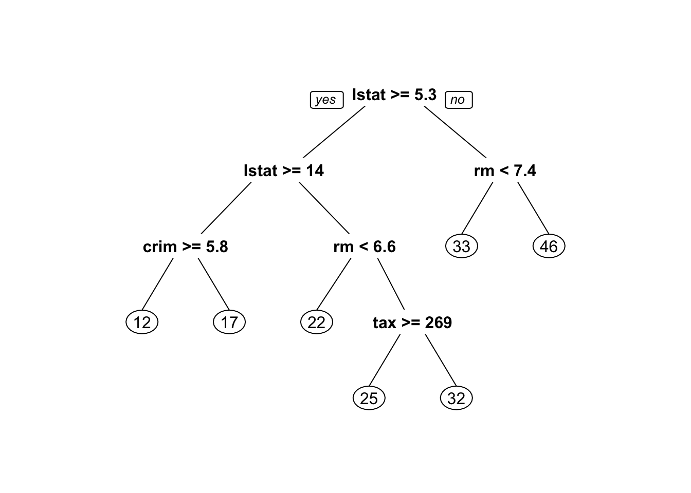

可以看出, 给定默认的参数时, rpart 返回的树 (包含7片叶子)比 tree 返回的树更小.

我们使用 prune 函数进行剪枝, 使用 prune 必须制定成本复杂度参数 cp. 对象 boston_tree 中的元素 cptable 已经储存了关于成本复杂度的信息.

min_cp = 
    boston_tree$cptable[
        which.min(boston_tree$cptable[,"xerror"]),
        "CP"]
min_cp

[1] 0.01419376

指定参数 min_cp 来进行剪枝:

boston_tree_prune = prune(boston_tree, cp=min_cp)
prp(boston_tree_prune)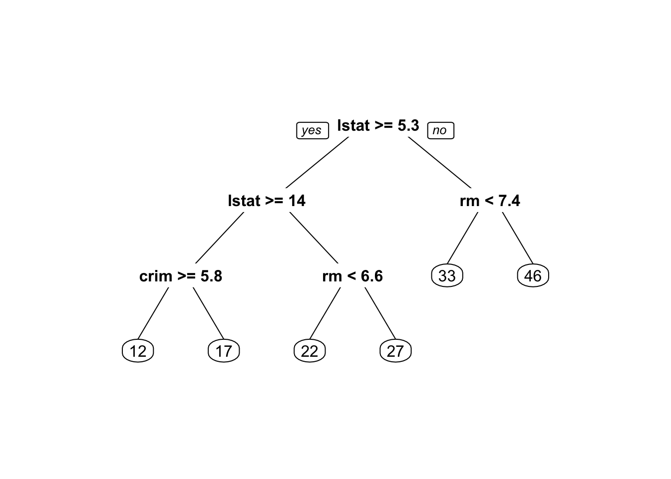

最后, 我们用 predict 函数来考察剪枝后的树 boston_tree_prune 的预测能力, 并和实际值对比:

boston_tree_tst_pred = predict(boston_tree_prune, newdata = boston_tst)
plot(boston_tree_tst_pred, boston_tst$medv, 
     xlab = "Predicted", ylab = "Actual", 
     main = "Predicted vs Actual: Single Tree, Test Data",
     col = "dodgerblue", pch = 20)
grid()
abline(0, 1, col = "darkorange", lwd = 2)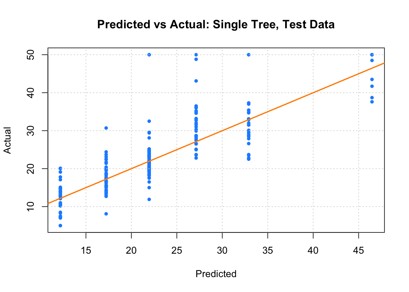

计算测试集上的 MSE:

mean((boston_tree_tst_pred - boston_tst$medv)^2)

[1] 28.01575

tree 包

rpart 包

`tree` 包

`rpart` 包