1 Introduction

Previously, we talked about the bias-variance tradeoff and briefly mentioned the James-Stein estimator. The main take-away is that a biased estimator may have a better performance than an unbiased estimator, in terms of achieving a lower MSE. In statistics, the most notable example is the James-Stein estimator.

We use R to demonstrate the superiority of James-Stein estimator for a particular model, which is also a good exercise for R programming and statistical computing.

2 Set-up

The hiring problem. Alice is a hiring manager. She looks at $N$ different aspects of each candidate’s characteristics (say communication skills, analytical skills, etc). A candidate’s true characteristic in aspect $i$ is $μ_i$. Alice cannot observe $μ_i$, but she can have an imperfect measure $z_i$ of each $μ_i$. Alice wishes to have a good estimate of a candidate’s characteristics $μ=(μ_1, \dots, μ_N)$ based on the measures $z = (z_1, \dots, z_n)$.

We build a simple model for the hiring problem:

• Data are generated from $$z_i | \mu_i \sim N (\mu_i, 1), \quad i = 1, \dots, N.$$

• In plain words, the first observation $z_1$ is drawn from the normal distribution with mean $μ_1$ and variance 1, the second observation $z_2$ is drawn from the normal distribution with mean $μ_2$ and variance 1, and so on.

• Note that for each candidate $\mu$, we have only one measurement $z$, which is composed of $N$ numbers, $(z_1,\dots, z_N)$.

Question: How to obtain a good estimate of $μ = (μ_1, \dots, μ_N)$ based on the one observation $z = (μ_1, \dots, μ_N)$?

1. The maximum-likelihood estimator (MLE) is $\hat{\mu}^{(MLE)} = z$. We can verify that this estimator is unbiased: $$\mathbb{E} \hat{\mu}^{(MLE)} = \mu.$$

2. The James-Stein Estimator is $\hat{\mu}^{JS} = (1- \frac{N-2}{||z||^2})z$.

Clearly, the James-Stein Estimator is biased. Indeed, it simply “shrinks” the unbiased MLE by $1- \frac{N-2}{||z||^2}$. When $N\ge3$, we have $1- \frac{N-2}{||z||^2} < 1$.

James-Stein Theorem (1961). For $N \ge 3$, the James-Stein Estimator dominates the MLE in terms of achieving a lower MSE: $$\mathbb{E} ||\hat{μ}^{(JS)} - μ||^2 < \mathbb{E} ||\hat{μ}^{(MLE)} - μ||^2,$$ where $||\hat{μ} - μ||^2 = \sum_{i=1}^N (\hat{μ}_i - μ_i) ^ 2$.

Proving this theorem may be thorny if you have limited exposure to mathematical statistics before. However, we can use R to run some experiments/simulations, and data will tell us whether this theorem holds in reality.

3 Experiments

The function run_experiment() performs the following operations:

1. Take an input N and generate some vector $μ$ with length N

2. Repeat the following steps nrep(=100) times:

   • generate a measurement z based on μ

   • compute the μ_MLE and μ_JSE based on z

   • compute the err_MLE and err_JSE based on z and μ

3. Return a data frame containing all the err_MLE and err_JSE

run_experiment = function(N) {
    nrep = 100
    err_MLE = rep(0,nrep)
    err_JSE = rep(0,nrep)
    μ = rnorm(N) # generated from standard normal dist
    
    for (i in 1:nrep) {
        e = rnorm(N,0,1)
        z = μ + e
        μ_MLE = z
        μ_JSE = (1-(N-2)/sum(z^2))*z
        err_MLE[i] = sum((μ_MLE-μ)^2)/N
        err_JSE[i] = sum((μ_JSE-μ)^2)/N
    }
    err_both = as.data.frame(cbind(err_MLE,err_JSE))
    names(err_both) = c("err_MLE","err_JSE")
    return(err_both)
}

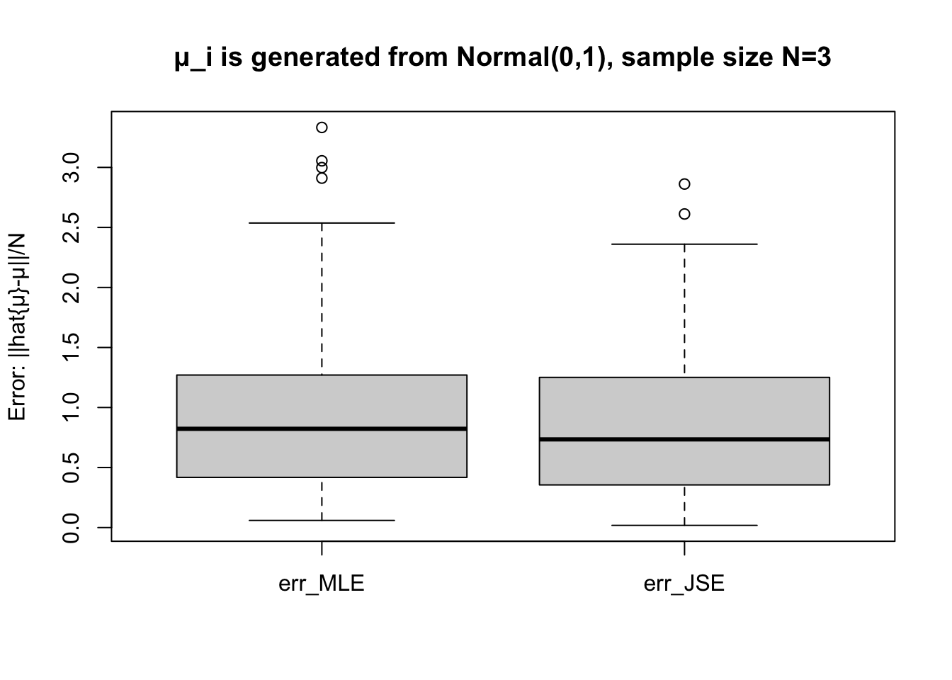
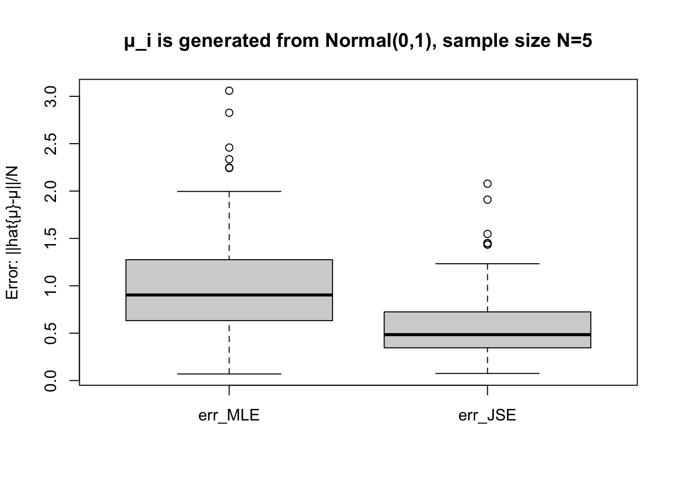
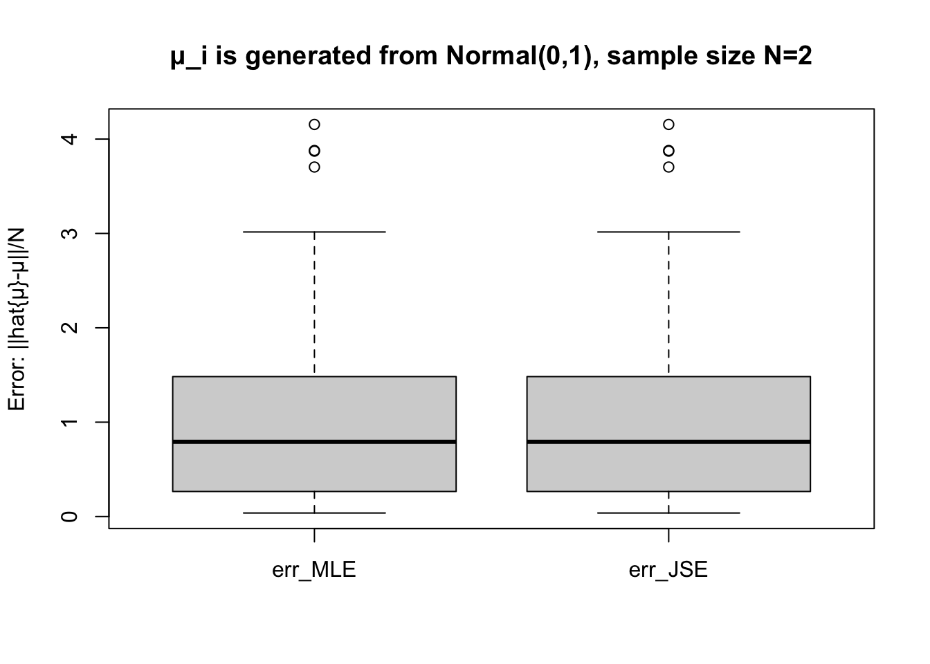
We have the data for all the MSEs on 100 samples of James-Stein estimator and Maximum Likelihood estimator. We use the box plot to compare them.

get_box = function(N) {
    err = run_experiment(N)
    boxplot(err, ylab = "Error: ||hat{μ}-μ||/N")
    title(paste("μ_i is generated from Normal(0,1), sample size N=",N,sep=""))
}

get_box(N=3)

get_box(N=5)

get_box(N=2)

The statistical experiments confirm the superiority of James-Stein estimator when $N \ge 3$.