library(ISLR)
library(ggplot2) # for plottingLogistic Regression Using Credit Card Data
Data
We will play with the simulated data set Default, from the ISLR package.
str(Default)'data.frame': 10000 obs. of 4 variables:
$ default: Factor w/ 2 levels "No","Yes": 1 1 1 1 1 1 1 1 1 1 ...
$ student: Factor w/ 2 levels "No","Yes": 1 2 1 1 1 2 1 2 1 1 ...
$ balance: num 730 817 1074 529 786 ...
$ income : num 44362 12106 31767 35704 38463 ...Default$default |> table()
  No  Yes
9667 333 - As you can see, the distribution of
defaultis very uneven. Just guessing “Yes” will be a pretty good prediction, with the accuracy rate being 96.7%.
ggplot(Default, aes(x=default)) +
  geom_bar()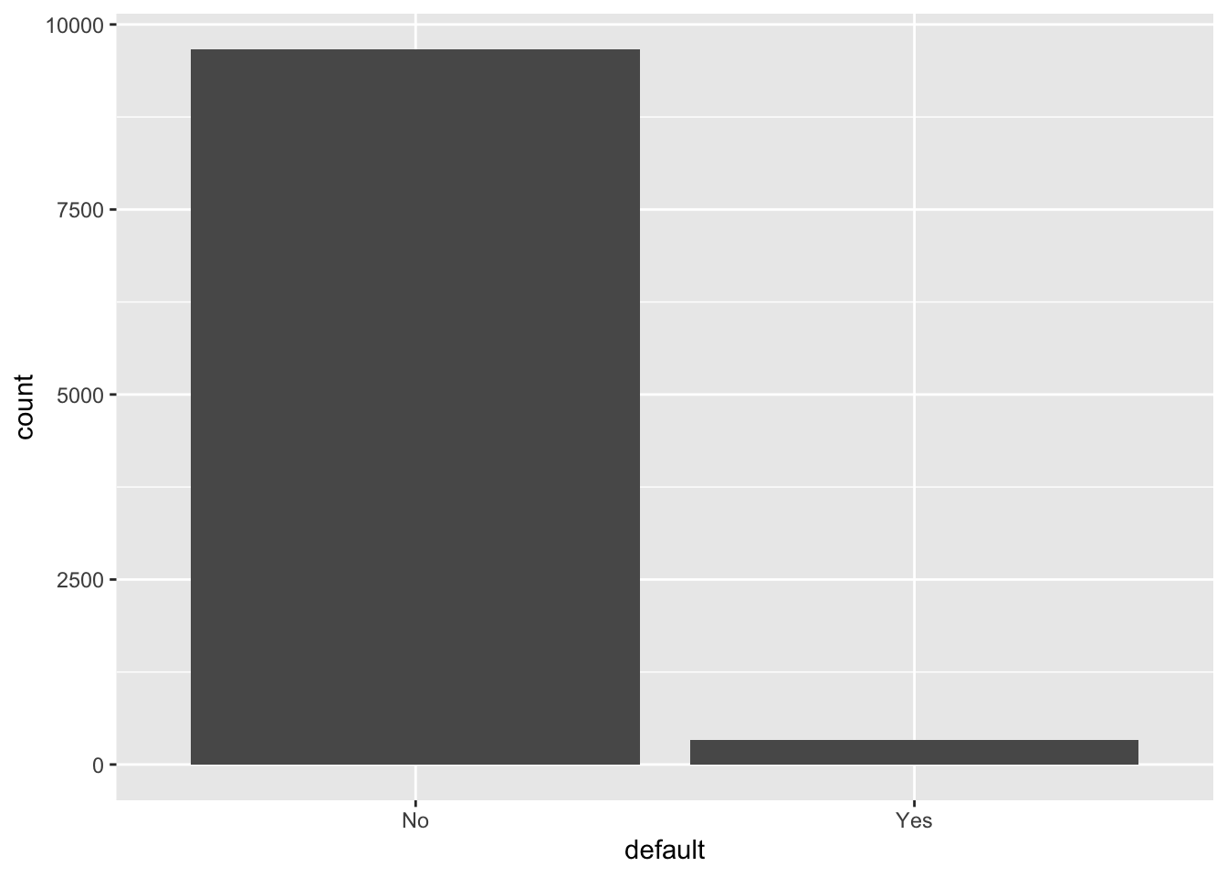
Logistic regression
glm.fit = glm(
    default ~ ., data = Default,
    family = "binomial")
summary(glm.fit)
Call:
glm(formula = default ~ ., family = "binomial", data = Default)

Coefficients:
              Estimate Std. Error z value Pr(>|z|)
(Intercept) -1.087e+01  4.923e-01 -22.080  < 2e-16 ***
studentYes  -6.468e-01  2.363e-01  -2.738  0.00619 **
balance      5.737e-03  2.319e-04  24.738  < 2e-16 ***
income       3.033e-06  8.203e-06   0.370  0.71152
---
Signif. codes:  0 '***' 0.001 '**' 0.01 '*' 0.05 '.' 0.1 ' ' 1

(Dispersion parameter for binomial family taken to be 1)

    Null deviance: 2920.6  on 9999  degrees of freedom
Residual deviance: 1571.5  on 9996  degrees of freedom
AIC: 1579.5

Number of Fisher Scoring iterations: 8
Remarks:
- As per the z-tests, all coefficients except that associated with
incomeare significant. - Unlike linear regression, we do not have an R-squared that tells us the fitness of our model. The alternative here is the AIC. The lower the AIC score, the better the fitness.
- However, for this course you should always use the training-validation-test datasets workflow for model selection and model testing. More on this later.
Evaluating the fitness: accuracy
Besides AIC, we can tell whether our model has a good fit by computing the accuracy rate.
Below we assume that our prediction of Default is “Yes” as long as Pr[Yes | X] > 0.5. Then, we compute the accuracy rate of our model under this decision rule (ie, predicting “Yes” as long as its estimated prob is higher than 0.5).
glm_pred_prob = predict(glm.fit, type="response")
glm_pred_outc = ifelse(glm_pred_prob>0.5, "Yes", "No")
mean(glm_pred_outc == Default$default)
[1] 0.9732- An accuracy rate of 97.3% looks very good.
- However, we know that a blind guess of “No” yields an accuracy rate of 96.7%. Also, considering that we are using the same data set for model fitting and model testing, it’s likely that our model is generally no better than a blind guess of “No.”
Two types of errors
In classification problems, we are usually concerned with the two types of error:
- False Positives (FP): the customer does NOT default, but the model incorrectly predicted the positive class (also known as a Type I error).
- False Negatives (FN): the customer DOES default, but the model incorrectly predicted the negative class (also known as a Type II error).
If we only look at the accuracy rate, we implicitly assume that Type I and Type II errors cause the same amount of loss to the decision maker. However, in this credit card problem, different banks may have different tolerances towards the two types of errors:
- For a small and growing bank which is trying to attract more customers, it cares more about the Type I error
- For a big bank that has lots of customers, it might care more about cost management and thus care more about the Type II error
table(glm_pred_outc, Default$default)
glm_pred_outc   No  Yes
          No  9627  228
Yes 40 105- Type I error rate: 40/(40+9627) = 0.41%
- Type II error rate: 228/(228+105) = 68.5%
So, a small bank that mainly cares about Type I error should like our model, but a big bank that mainly cares about Type II error should not.
As a comparison, the blind guess of “No” has accuracy 96.7, Type I error rate 100% and Type II error rate 0%. Indeed, in this credit card problem, a blind prediction of “No” might be a very good decision rule for a small bank that is trying to attract more customers.
ROC curve
You should have noticed that there is a tradeoff between Type I error rate and Type II error rate at varying threshold values. Intuitively, we should predict “Yes” when the estimated probability is above some threshold: \[ \textrm{``Yes'' if } \Pr [Y_i | X_i] \ge p^* \]
- When \(p^* = 0\) (ie, always say “Yes”), Type I error rate is zero and Type II error rate is 100%.
- When \(p^* = 1\) (ie, always say “No”), Type I error rate is 100% and Type II error rate is zero.
- The optimal \(p^*\) depends on the domain knowledge. After all, we must know the exact costs associated with each type of error to determine the optimal threshold.
The ROC curve plots the true positive rate (TPR, or \(1-\) Type II error rate) against the false positive rate (FPR, or Type I error rate) at each threshold setting.
- The naming of the ROC curve is historical and comes from the communication theory.
Below are some examples of the ROC curve.
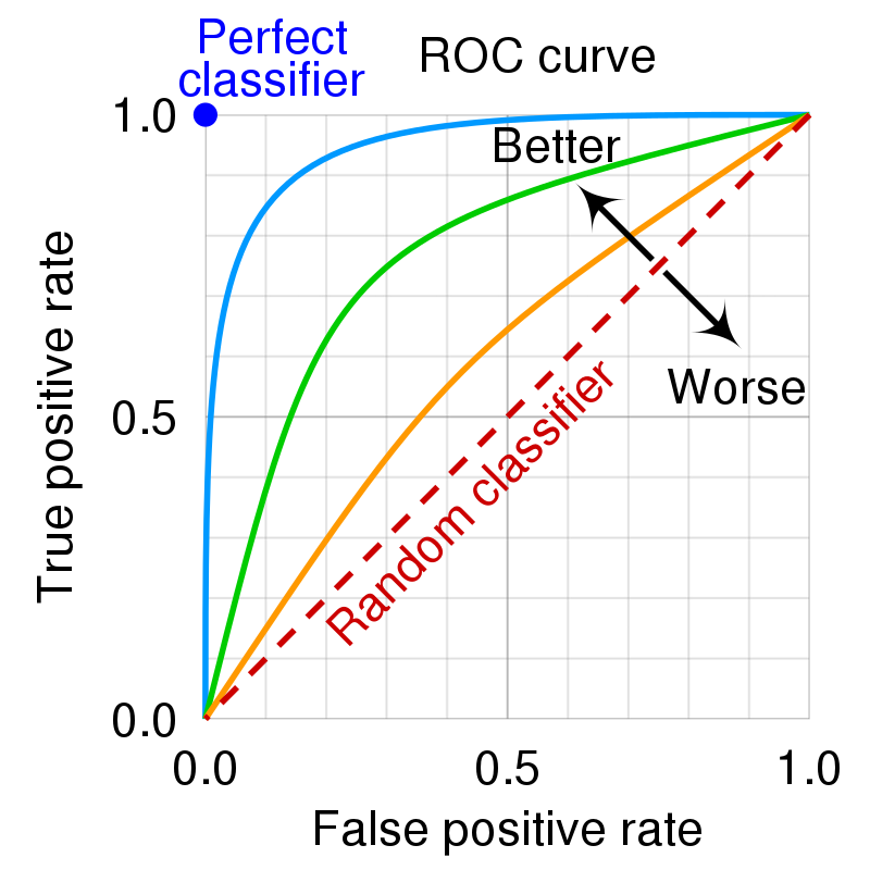
- An ideal ROC curve will hug the top left corner.
- The overall performance of our model can be judged by the area under the ROC curve. This area is called AUC (Area Under Curve).
Below we plot the ROC curve and compute the AUC for our model.
library(pROC)
roc_logistic <- roc(Default$default ~ glm_pred_prob) # true outcomes against our predicted probabilities
g <- ggroc(roc_logistic, legacy.axes=TRUE)
g + xlab("False Positive Rate") + ylab("True Positive Rate")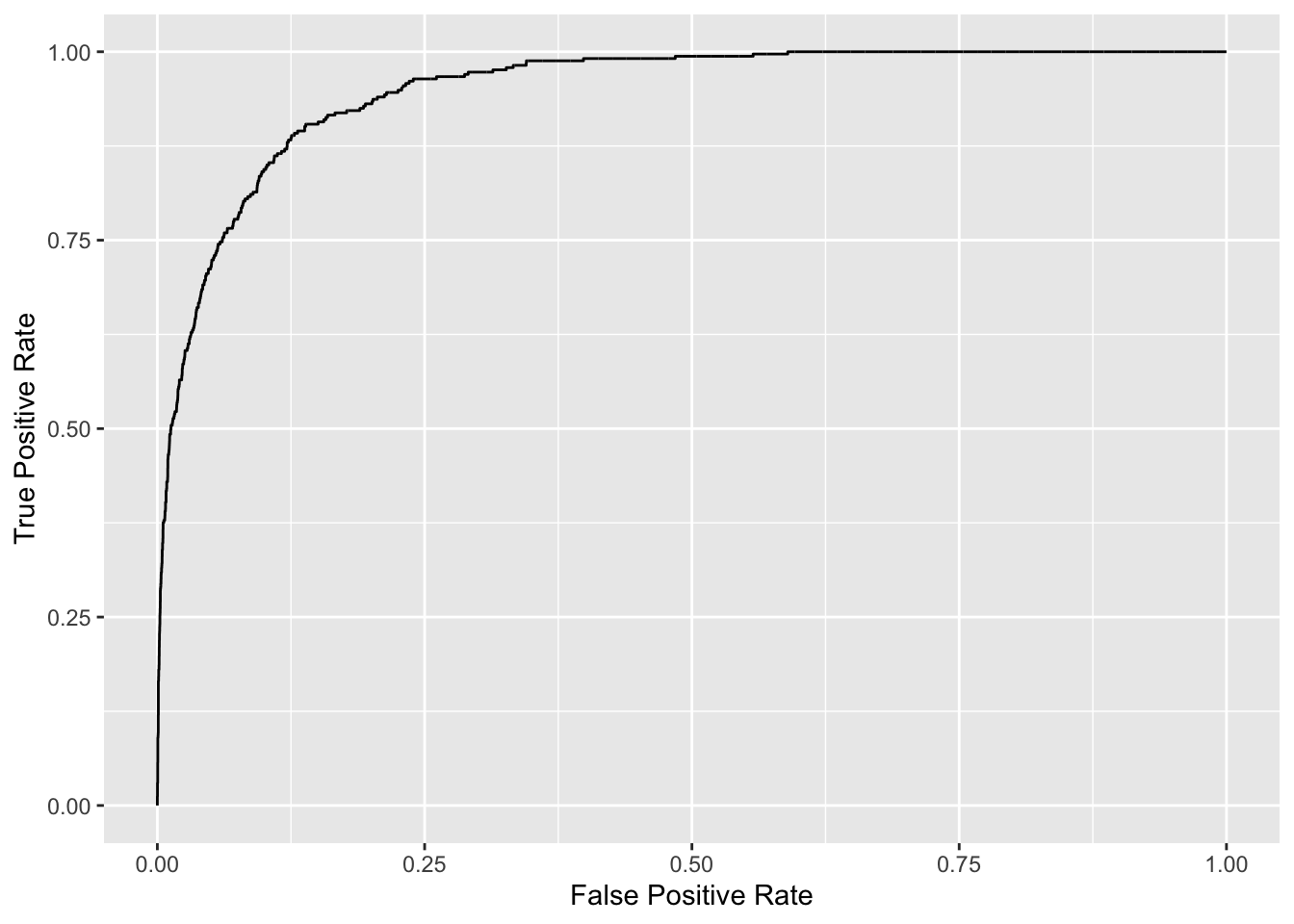
# get auc
auc(roc_logistic)
Area under the curve: 0.9496