library(dplyr) # for data wrangling
library(ggplot2) # for plottingLogistic Regression, KNN and LDA
Stock Market Data
We will play with the Smarket dataset, bundled in the ISLR package.
library(ISLR)I tend to use the str function (short for “structure”) whenever I encounter a new R object. A good thing about the str function is that it works with all R objects (functions, vectors, lists, etc).
str(Smarket)'data.frame': 1250 obs. of 9 variables:
$ Year : num 2001 2001 2001 2001 2001 ...
$ Lag1 : num 0.381 0.959 1.032 -0.623 0.614 ...
$ Lag2 : num -0.192 0.381 0.959 1.032 -0.623 ...
$ Lag3 : num -2.624 -0.192 0.381 0.959 1.032 ...
$ Lag4 : num -1.055 -2.624 -0.192 0.381 0.959 ...
$ Lag5 : num 5.01 -1.055 -2.624 -0.192 0.381 ...
$ Volume : num 1.19 1.3 1.41 1.28 1.21 ...
$ Today : num 0.959 1.032 -0.623 0.614 0.213 ...
$ Direction: Factor w/ 2 levels "Down","Up": 2 2 1 2 2 2 1 2 2 2 ...Knowing that Smarket is a data frame, we can apply the head function to it:
head(Smarket) Year Lag1 Lag2 Lag3 Lag4 Lag5 Volume Today Direction
1 2001 0.381 -0.192 -2.624 -1.055 5.010 1.1913 0.959 Up
2 2001 0.959 0.381 -0.192 -2.624 -1.055 1.2965 1.032 Up
3 2001 1.032 0.959 0.381 -0.192 -2.624 1.4112 -0.623 Down
4 2001 -0.623 1.032 0.959 0.381 -0.192 1.2760 0.614 Up
5 2001 0.614 -0.623 1.032 0.959 0.381 1.2057 0.213 Up
6 2001 0.213 0.614 -0.623 1.032 0.959 1.3491 1.392 UpSmarket provides the daily percentage returns for the S&P 500 stock index between 2001 and 2005. Run ?Smarket to read the manual.
As the output of str(Smarket) shows, the variable Smarket$Direction is an R factor, used mainly for categorical data.
str(Smarket$Direction) Factor w/ 2 levels "Down","Up": 2 2 1 2 2 2 1 2 2 2 ...- Here
Directionhas two levels: Down and Up.
summary(Smarket$Direction)Down Up
602 648 We will use several classification models to predict whether the market will go up or down tomorrow (ie, the value of Direction). Possible features for predicting include:
Volume: Volume of shares traded in billionsLag1toLag5: Percentage return for previous day, 2 days previous, …, 5 days previous
Data wrangling and plotting
Each individual variable in Smarket is actually time series data, from year 2001 to year 2005. Let’s plot the time trend of Volume:
ggplot(
    Smarket,
    aes(x=seq(dim(Smarket)[1]), y=Volume)
    ) + geom_line() + xlab("Day")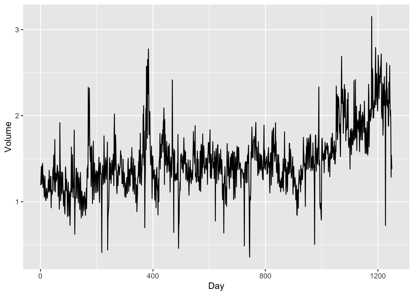
- There is an increasing trend in
Volumeas more and more investors participate in the stock market.
Now let’s see whether there is a time trend in the stock returns.
ggplot(
    Smarket,
    aes(x=seq(dim(Smarket)[1]), y=Today)
    ) + geom_line() +
    ylab("Percentage return") + xlab("Day")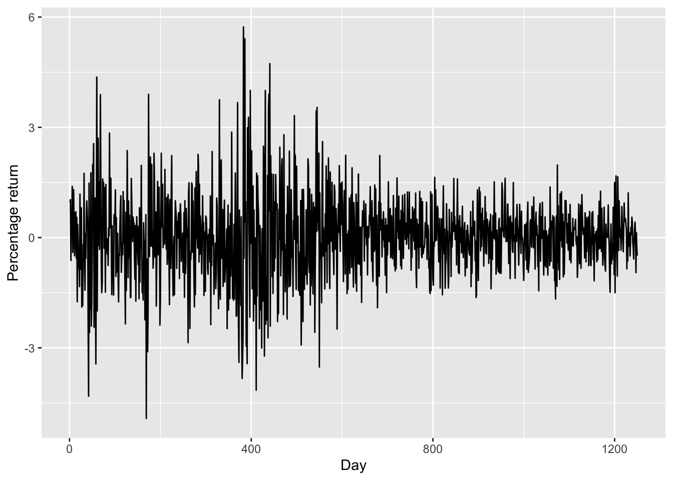
- There is no increasing or decreasing trend in stock price (
Today). - The plot also suggests that the stock prices are much more volatile between day 0 to day 600. This is probably due to the dot-com bubble as day 0 is the start of 2001.
Then, let’s plot the Lags against Direction. At the same time, we also encode “Up” and “Down” as “1” and “-1” respectively, and add the fitting lines. The reason is that there are two “theories” about how the stock price today will affect its price tomorrow: the momentum effect and the reversal effect.
library(reshape2) ## for melting data later

smarket_melt <- Smarket |>
    dplyr::mutate(Direction = if_else(Direction == "Up", 1, -1)) |>
    dplyr::select(starts_with(c("Lag", "Direction"))) |>
    reshape2::melt(id="Direction")

ggplot(
  smarket_melt,
  aes(x = value, y = Direction)) +
    facet_wrap(~variable, scales="free") +
    geom_point() +
    geom_smooth(method = "lm")
`geom_smooth()` using formula = 'y ~ x'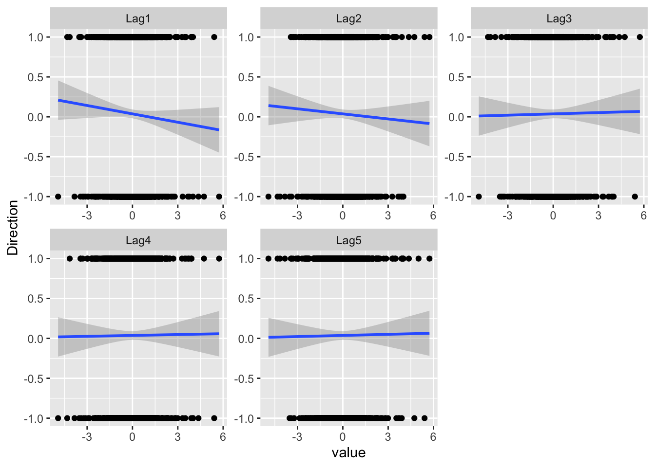
- For Lag1 and Lag2, the fitted lines are downward-sloping, suggesting that the reversal effect might exist for our data.
- The lagged prices from Lag3 seem to have little predictive power.
Based on the exploratory studies (and some basic knowledge about stock markets), we use Lag1, Lag2 and Volumn for predicting Direction. Let’s create a new data frame df containing only these variables.
df = as_tibble(Smarket) |>
    select(Lag1, Lag2, Volume, Direction)
Logistic regression
We use the glm function to perform the logistic regression. To do that, we must pass in the argument family=binomial, and the rest is similar to what we do with the lm function:
glm.fits = glm(Direction ~ ., data=df, family=binomial)summary(glm.fits)
Call:
glm(formula = Direction ~ ., family = binomial, data = df)

Coefficients:
            Estimate Std. Error z value Pr(>|z|)
(Intercept) -0.12058    0.24018  -0.502    0.616
Lag1        -0.07326    0.05017  -1.460    0.144
Lag2        -0.04279    0.05006  -0.855    0.393
Volume       0.13184    0.15799   0.835    0.404

(Dispersion parameter for binomial family taken to be 1)

    Null deviance: 1731.2  on 1249  degrees of freedom
Residual deviance: 1727.7  on 1246  degrees of freedom
AIC: 1735.7

Number of Fisher Scoring iterations: 3
Remarks on the regression result:
The z value is computed by
EstimateoverStd. Error. The z-statistic obeys the standard normal distribution, which is somewhat simpler than the t-distribution as used in significance tests of linear regression. Since we use MLE in logistic regressions, the nice properties of the likelihood function contribute to this simplification.The smallest p-value is associated with
Lag1, with the p-value being about 0.14. As the p-value is still relatively large, there is no clear evidence of a real association betweenLag1andDirection.
How well does our logistic model perform?
Given the fitted model glm.fits, a natural question is how well our model performs compared to a random guess of “Up” and “Down.”
Given fixed values of the predictors, we can use the predict function to predict the probability that the market will go up (ie, \(\Pr [Y = 1 | X]\)). When we do not specify the values of the predictors, predict will automatically use the training data contained in the fitted glm model:
glm.probs = predict(glm.fits, type="response")- The option
type = responseensures that the outputs are probabilities rather than the logits (\(\textrm{Logit} (P) = \log( P / (1−P))\)). - Here
glm.probsare the predicted probabilities of the market going up, \(\Pr [Y = 1 | X]\).
str(glm.probs) Named num [1:1250] 0.504 0.491 0.487 0.512 0.505 ...
- attr(*, "names")= chr [1:1250] "1" "2" "3" "4" ...Then, we convert these predicted probabilities to Up/Down.
glm.pred = if_else(glm.probs > 0.5, "Up", "Down")- The
if_elseis a handy command for creating a vector that takes conditional values.
head(glm.pred)[1] "Up" "Down" "Down" "Up" "Up" "Up" Now compare our predictions glm.pred with the true directions.
mean(glm.pred == df$Direction)[1] 0.5312- It seems our model works better than a random guess: 0.5312 > 0.5. Cool!
To evaluate the performance of a classification algorithm, we can also use the so-called “confusion table.” The confusion table is composed of:
- True Positives (TP): These are instances where the model correctly predicted the positive class.
- True Negatives (TN): These are instances where the model correctly predicted the negative class.
- False Positives (FP): These are instances where the model incorrectly predicted the positive class (also known as a Type I error).
- False Negatives (FN): These are instances where the model incorrectly predicted the negative class (also known as a Type II error).
As the confusion table is widely used in statistics, R provides the table function just for making the confusion table:
table(glm.pred, df$Direction)
glm.pred Down  Up
    Down  147 131
Up 455 517- The diagonal elements of the confusion matrix indicate correct predictions, while the off-diagonals represent incorrect predictions.
- It looks like our model gives a better prediction when the market goes Up than when the market goes Down.
Training data and hold-out data
However, we know that the comparison above is misleading as we are using the same data for model training and model testing. In order to better assess the accuracy of the logistic regression model, we should fit the model using part of the data, and then examine how well it predicts the hold-out data.
We use the observations from 2001 through 2004 as training data.
train = (Smarket$Year < 2005)- The object
trainis a boolean vector for specifying the training dataset fromdf. The training data will bedf[train, ]and the hold-out set will bedf[!train ,].
Fit our model on the training data. Note the option subset=train:
glm.fits = glm(
    Direction ~ .,
    data=df[train, ],
    family=binomial)
Test our model performance on the hold-out data:
glm.probs = predict(
    glm.fits, df[!train, ],
    type="response")
Convert the predicted probabilities to Up/Down:
glm.pred = if_else(glm.probs > 0.5, "Up", "Down")Compute the accuracy rate:
mean(glm.pred == df[!train, ]$Direction)[1] 0.4761905- It turns out that our model is no better than random guessing.
This result is disappointing, but reasonable. One should not expect to predict future market performance using past returns solely.
K-Nearest Neighbors
To perform KNN, We use the knn function from the class package.
library(class)The usage of knn is distinct from lm/glm in that the steps of model fitting and model predicting ( or testing) are bundled in the same command. Specifically, knn requires four inputs:
- a matrix containing the predictors for model fitting (
train.Xbelow). - a matrix containing the predictors for which we wish to make predictions (
test.Xbelow) - a vector containing the class labels for the training observations (
train.Directionbelow)
train.X = cbind(df$Lag1, df$Lag2)[train ,]test.X = cbind(df$Lag1, df$Lag2)[!train,]train.Direction = df$Direction[train]Before using the knn function, we should set a random seed. The reason is that when several observations are tied as nearest neighbors, R will randomly break the tie. Therefore, a seed must be set in order to ensure reproducibility of results.
set.seed(1)
knn.pred = knn(
    train.X, test.X,
    train.Direction, k=1)
mean(knn.pred == df$Direction[!train])
[1] 0.5- The results using
k=1are not good, as the prediction accuracy is only 50%. - The option
k=1means that we only consider one nearest neighbour, which will lead to an overly flexible fit.
Below, we repeat the analysis using k=3:
knn.pred = knn(
    train.X, test.X,
    train.Direction, k=3)
mean(knn.pred == df$Direction[!train])
[1] 0.5357143- The results have improved slightly. But increasing \(K\) further turns out to provide no further improvements.
Linear Discriminant Analysis
We fit an LDA model using the lda function, which is part of the MASS package. Unlike knn, the syntax of lda is very similar to that of lm/glm.
lda.fit = MASS::lda(Direction ~ Lag1+Lag2,
              data=Smarket, subset=train)
lda.fit
Call:
lda(Direction ~ Lag1 + Lag2, data = Smarket, subset = train)
Prior probabilities of groups:
Down Up
0.491984 0.508016
Group means:
Lag1 Lag2
Down 0.04279022 0.03389409
Up -0.03954635 -0.03132544
Coefficients of linear discriminants:
LD1
Lag1 -0.6420190
Lag2 -0.5135293In the LDA output, the prior probabilities are \(π^1 = 0.492\) and \(π^2 = 0.508\). That is, in 50.8% of the training observations the market goes up.
mean(df$Direction[train] == "Up")[1] 0.508016The group means are the average of each predictor within each class, which are used as estimates of \(\mu_k\).
df[train, ]# A tibble: 998 × 4
Lag1 Lag2 Volume Direction
<dbl> <dbl> <dbl> <fct>
1 0.381 -0.192 1.19 Up
2 0.959 0.381 1.30 Up
3 1.03 0.959 1.41 Down
4 -0.623 1.03 1.28 Up
5 0.614 -0.623 1.21 Up
6 0.213 0.614 1.35 Up
7 1.39 0.213 1.44 Down
8 -0.403 1.39 1.41 Up
9 0.027 -0.403 1.16 Up
10 1.30 0.027 1.23 Up
# ℹ 988 more rowsNow we test the performance on the hold-out set:
lda.pred = predict(lda.fit, df[!train, ])
names(lda.pred)
[1] "class" "posterior" "x" The predict function returns a list with three elements:
- class, LDA’s predictions about the movement of the market
- posterior, a matrix whose k-th column contains the posterior probability that the corresponding observation belongs to the k-th class
x: the linear discriminants.
mean(lda.pred$class == df[!train, ]$Direction)[1] 0.5595238- So far, LDA has the best performance.
Besides a simple Up-or-Down prediction, sometimes we want to know whether the market is very likely to go up. For instance, we may want to predict a market decrease (and short the market) only when the posterior is at least 90%:.
However, no days in 2005 meet that threshold. In fact, the greatest posterior probability of decrease in all of 2005 was about 52.0%.
lda.pred$posterior[, 1] |> max()[1] 0.520235- This result is consistent with the so-called efficient market hypothesis, which claims that we cannot use the past stock prices to predict the future stock prices.